Whenever I encounter complex mathematical objects, the initial question that arises in my mind is: how does this relate to the natural world? I must admit, I thoroughly enjoy exploring abstract concepts for the sheer joy of their complexity. Nevertheless, it can be incredibly enlightening to witness these abstractions manifesting in real-life scenarios.
Today, I am excited to share an intriguing discovery I came across through this article: On the Local Behavior of Spaces of Natural Images. Although this is an aged finding, it continues to captivate me. The authors of this research demonstrated that the Klein bottle can be found right in our surroundings — specifically, in photographs taken outdoors. It may sound puzzling, but the crux of the matter is this: the fundamental building blocks of images captured under natural outdoor lighting can be attributed to the structure of the Klein bottle. If this piques your curiosity, I invite you to delve deeper into the subject.
Before we proceed, it is essential to clarify a few aspects. We will exclusively work with monochromatic images, meaning that all images will be represented in shades of grey. Additionally, when we refer to building blocks, we are specifically focusing on small patches measuring 3x3 pixels. This is an example of such patch:

Indeed, every image can be broken down into these fundamental building blocks. Picture an artist meticulously creating a photo-realistic landscape using a pointillist style, similar to the artist depicted below (I’m not very good at drawing):

As the artist dips their brush into the palette of colors, they are actually accessing a set of patches like this:

Typically, artists organize their palettes on a flat piece of wood or plastic, which is practical to prevent the paints from spilling onto the ground. However, in our case, these patches inhabit a more fascinating object. Now, the question arises: How can we detect the presence of this intriguing object?
To begin our exploration, we associate each patch with a point in a 9-dimensional vector space. Our focus is on identifying the brightest patches, technically speaking. For this purpose, we calculate the intensity of each pixel within the patch and then evaluate a specific D-norm on the vector of these intensity values. Our main interest lies in the upper quantile of these patches concerning the value of this norm. After applying appropriate normalization techniques, we obtain points that lie on a 7-dimensional ellipsoid.
Please, don’t be intimidated! The key point to remember is that most intriguing curves and surfaces on this 7-dimensional ellipsoid turn out to be surprisingly straightforward.
Now, let’s delve into an interesting question: Are all the patches distributed evenly on this ellipsoid? It turns out that they are not. By isolating the most densely populated points on the ellipsoid, we can observe the shape they collectively form. Surprisingly, these points trace out a closed curve, or more simply, a circle. We’re going to draw this circle along with the patches from the densest points. Make note that we will depict the patches in a smoothed-out form, in accordance with the paper’s methodology:

The circle formed by the densely populated points on the 7-dimensional ellipsoid is named S_lin because of its interesting property: you can move around the circle using linear transformations. This is fascinating because despite the vast variety of possible patches, the most commonly used and noticeable ones (considering intensity filtration) lie within this circular gradient.
In summary, we have discovered that the most common patches in this 9-dimensional space actually form a circle, lying on a 7-dimensional sphere. However, you might be wondering, where does the Klein bottle come into play? Well, here’s the catch: the number of most crowded points we include was somewhat arbitrary. We can experiment with this number until we end up with something like this:

We get several glued circles which we will cal following the paper: Sₗᵢₙ, Sₕ, and Sᵥ. It’s important to observe that the Sₕ and Sᵥ circles do not intersect, yet they both exist on the same 7-dimensional sphere. High-dimensional geometry is very weird most of the times.
The resulting structure is known as the “3-circle”. Now it is worthwhile to examine the inner structures of these loops and plot patches from the densest points along these circle, resulting in the following representations:


Every loop depicts a certain gradient: vertical, horizontal and circular! Now it becomes evident why the authors chose to use these lowercase indices in their notation. If we refer back to artist metaphor, each loop corresponds to a specific section of the artist’s palette, describing a certain gradient. This way of organizing paints suggests that the “artist” conceives paintings in terms of linear transformations.
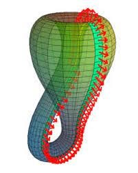
But we’re not done yet. If we increase the number of densest points further, we encounter a very peculiar object that is difficult to depict in a similar manner. So, first, let’s break up our circles:

Let’s visualize the lower and upper edges of our picture as glued together, while keeping our circles intact. This aspect is evident in our picture: you’ll notice that the upper and lower patches on both circles are identical.
Next, we need to represent Sₗᵢₙ in a more intricate way. It will be broken up, and its patches will populate two rows simultaneously:

Observe that the blue Sₗᵢₙ circle first moves from right to left along the second row, then wraps around the scene and repeats the motion from right to left along the fourth row. The similarity of patches along its path signifies gluing points.
Now, let’s revisit the original problem. We can fill this picture with the next set of densely populated points:

You can see how new patches fall into place and compliment existing gradient patterns. They also fill in the the inner parts of the circles, so what we have on our hands is now a 2-dimensional shape instead of 1-dimensional. Moreover, these new patches align with what was already going on edge-wise. The lower and upper edges virtually “glued” and are identical, as we previously discussed. If the left and right edges were also identical, this object would describe a typical 2-dimensional torus. However, they are not exactly the same; they exhibit a twist, which is signified by reversed directions of arrows. This precisely characterizes the Klein bottle!

If you are intrigued by the details, I strongly recommend referring to the original paper: On the Local Behavior of Spaces of Natural Images. It delves deeper into the subject, providing a comprehensive understanding of the mathematical framework used to establish the object’s classification as a Klein bottle. However, it is worth noting that the paper may require some familiarity with concepts such as persistence diagrams and density estimators to grasp the methodology fully. Additionally, delving into algebraic concepts might be necessary to understand how precisely this Klein bottle is differentiated from a torus.